
A repository for a Graphical User Interface for supervised and unsupervised image classification for Bio7 which can be extended easily.
The classification plugin and dependencies are shipped since Bio7 3.2. The plugin can be started in the R-Shell view context menu ("Image Classification->Main").
You can also use this repository (with the Eclipse EGit plugin - available in the Update Manager of Bio7) to download, compile and start the latest version of this plugin.
ImageJ updates are available via an Update Site (Menu: "Help->Install New Software...") default available in the Update Manager since Bio7 3.2.
At first start the plugin is compiled to Java classfiles (*.class). For distribution just copy all new sources in the plugin install directory (delete the old plugins *.java and *.class files)!
The Graphical User Interface was created with the Eclipse Window Builder which can be installed into Bio7. Open the file _ModelGui.java with WindowBuilder to edit or customize the GUI.
First steps:
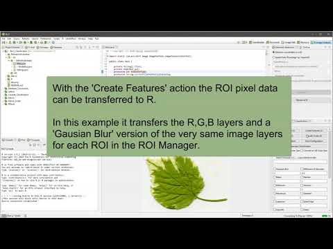
Classification preview from a selection:

With the "Create Classification Project" wizard action a classification Bio7 project can be created with an optional folder structure. The default R templates can be copied to the new project location for custom scripts (paths have to be adjusted and stored in a configuration file - see below!).
Open an image in ImageJ and follow Button 1-4 for a classification workflow which trains and classifies images with R (scripts are available in the R directory) in a non-blocking job. For an unsupervised classification (e.g., k-means) just use the classification action (4).
RGB images can be converted to a different color space (see option HSB Stack, LAB Stack) and selected channels from multichannel images or stacks can be extracted individually.
Several features can be enabled in the default tab which will be added to the default image layers. A comma separated text argument adds filter images of different radius or applies special settings for edge algorithms like Difference of Gaussian, Lipschitz, Gabor, Convolve. For some edge detection methods a ';' separator can be set, too, for different sets of edge settings (Difference of Gaussian, Lipschitz, Gabor, Convolve) resulting in one image layer each.
The filters and features are described in the "Filters and Features Guide" below.
All filters are computed in parallel (each filter layer is a task, the texture measures are also computed row by row in parallel). The Kuwahara filter works with float images (formerly the bits of the float pixels were read as integers) and the Lipschitz filter uses a fixed range for the conversion to 8-bit (the same for a preview and the complete image) - models trained with these layers should be trained again.
All settings for classification can be stored or reopened with the 'Load/Save Configuration' actions in a simple text file (simply drag the file on the GUI interface to load it!).
Each enabled filter adds one or more layers (for each selected channel) to the feature stack which is used for the pixel classification. Options are separated with ',' (e.g., several radii, each adds a layer) and several sets of settings with ';'. Small radii and sigmas describe fine details, large ones the context of a pixel. A combination of a few scales (e.g., 1,2,4,8) of a few filter types usually works better than many filters of one scale. The option fields and the check boxes have tooltips with a short description.
| Option | What it does | Suited for |
|---|---|---|
| Convert to HSB | Hue, saturation and brightness channels of RGB images | Objects which differ in color but not in brightness (e.g., plant tissue, stained cells, vegetation) |
| Convert to LAB | Perceptually uniform L, a, b channels of RGB images | Color segmentation independent of the illumination (L = lightness, a = green-red, b = blue-yellow) |
| Select Channels | Only the given channels or slices are used (e.g., 1,3) | Removing channels without information (less layers, faster) |
| Filter | What it computes | Option (example) | Suited for |
|---|---|---|---|
| Gaussian Blur | Gaussian smoothed image (sigma * 0.4 as in Weka) | sigmas (2,4,8) | Noise reduction, the intensity at different scales (background, large objects) |
| Mean | Mean in a circular neighborhood | radii (2) | Smoothing, local brightness |
| Median | Median in a circular neighborhood | radii (2) | Salt and pepper noise, smoothing with sharp edges |
| Minimum, Maximum | Minimum or maximum in a neighborhood | radii (2) | Dark or bright small structures, gaps, the morphological context |
| Variance | Variance in a neighborhood | radii (2) | Textured vs. smooth regions, edges |
| Top Hat | Image minus its morphological opening | radii (2) | Small bright objects (spots, nuclei, particles) on an uneven background |
| Kuwahara | Mean of the quadrant with the smallest variance | window sizes (5) | Edge preserving smoothing, homogeneous regions with sharp borders |
| Bilateral | Smoothing weighted by distance and value difference | spatial sigma,range sigma relative to the value range (3,0.1) | Edge preserving noise reduction (cells, tissue borders, remote sensing) |
| Anisotropic Diffusion | Perona-Malik diffusion which stops at edges | iterations,kappa relative to the value range,lambda (10,0.1,0.2) | Strong noise with important borders, smooth regions (e.g., medical or SEM images) |
| Filter | What it computes | Option (example) | Suited for |
|---|---|---|---|
| Difference of Gaussian | Difference of two Gaussian blurred images (band pass) | sigma1,sigma2 - sets with ';' (2,4;4,8) | Blobs and structures of a certain size, spots |
| Gradient | Sobel derivative in x and y direction (optional of Gaussian blurred images) | sigmas or empty (1,2) | Edges with a direction |
| Gradient Magnitude | Strength of the gradient of the Gaussian blurred image | sigmas (1,2) | Object borders independent of the direction, boundary detection |
| Laplacian | Second derivative (optional of Gaussian blurred images = LoG) | sigmas or empty (2) | Blobs, spots and thin lines, zero crossings at edges |
| Sobel Edge | Edge magnitude of ImageJ (Find Edges, optional blurred) | sigmas or empty | Edges, borders |
| Hessian | Largest and smallest eigenvalue and the determinant of the Hessian matrix | sigmas (1,2) | Blobs (both eigenvalues large), ridges, vessels, filaments, membranes (one large eigenvalue) |
| Structure Tensor | Largest and smallest eigenvalue and the coherence of the local gradients | gradient sigma,integration sigma - sets with ';' (1,3) | Oriented textures (fibres, wood, muscle, stripes, fingerprints), corners and edges |
| Lipschitz | Lipschitz cover filters (top hat / down hat) | down,top,slope - sets with ';' (true,true,10) | Uneven background, spots and small structures with a slope |
| Convolve | Convolution with an own kernel (ImageJ syntax) | kernel - sets with ';' | Own filters (e.g., special edge, line or spot detectors) |
| Filter | What it computes | Option (example) | Suited for |
|---|---|---|---|
| Gabor | Response of an oriented Gabor filter (wavelength, orientation) | size,wavelength,orientation,phase,sigma,aspect ratio - sets with ';' (3,4.0,0.6,1.0,2.0,0.3) | Periodic and oriented textures with a known scale and direction (fabric, cells in rows, ripple patterns) |
| Haralick Texture (GLCM) | Texture features of the gray level co-occurrence matrix in a window (see below) | window widths, distances, gray levels | Regions which are separated by their texture and not by the brightness (tissue types, land cover, materials, surfaces) |
| Local Entropy | Entropy of the histogram in a window | radii (3,5) | Textured vs. smooth regions, the complexity of a region |
| Local Binary Pattern | Rotation invariant uniform LBP code (edges, corners, spots, flat areas) | radii (1,2) | Micro textures independent of the illumination (surfaces, cells, skin, materials) |
| Laws' Texture Energy | 9 rotation invariant energy maps of the 5x5 Laws masks (L = level, E = edge, S = spot, R = ripple) | radius of the energy window (7) | Classic texture classification: edge, spot and ripple textures (materials, terrain, histology) |
The Haralick features (Haralick et al. 1973) of the co-occurrence matrix of the gray levels in all four directions:
| Feature | Meaning | Suited for |
|---|---|---|
| ASM (Energy) | Uniformity of the texture (high for homogeneous regions) | Homogeneous vs. textured regions |
| Contrast | Local intensity variations | Rough vs. smooth textures, borders |
| Correlation | Linear dependency of the gray levels of the pixel pairs | Regular and oriented structures |
| Variance | Dispersion of the gray levels | Heterogeneous regions |
| IDM (Homogeneity) | Inverse difference moment (high for small differences) | Smooth regions, similar to ASM |
| SumAverage, SumVariance, SumEntropy | Statistics of the sums of the pixel pairs | Brightness and its variation in the texture |
| Entropy | Randomness of the texture | Complex, irregular textures |
| DiffVariance, DiffEntropy | Statistics of the differences of the pixel pairs | Fine textures, edges |
| IMC1, IMC2 | Information measures of the correlation | Dependencies of the gray levels independent of the brightness |
The window should be larger than the texture pattern (e.g., 7-15), the distance smaller than the pattern (1-3). 32 gray levels are a good compromise (more levels need larger windows). "Select Typical" selects ASM, Contrast, Correlation, IDM and Entropy. The gray levels are quantized in fixed ranges (8-bit and RGB: 0-255, HSB: 0-1, LAB: L 0-100, a, b -128-128, else the display range) that a preview of a selection and the complete image use the same levels.
| Filter | What it computes | Option (example) | Suited for |
|---|---|---|---|
| Neighbors | The values of the 8 neighbors at a distance | distances (1,4) | The context of a pixel: thin structures, object borders, the position relative to other objects |
| Membrane Projections | A line rotated in 30 orientations: Mean, Max, Min, Sum, Std and Median of the responses | patch size,thickness (19,1) | Membranes, cell borders, fibres, vessels, roads and other thin linear structures in any orientation |
- Brightness or color differences: Gaussian Blur and Mean at a few sigmas, HSB or LAB for color images.
- Spots, nuclei, particles: Difference of Gaussian, Laplacian, Hessian, Top Hat.
- Borders, membranes, filaments: Gradient Magnitude, Hessian, Membrane Projections, Structure Tensor.
- Textured regions (tissue types, materials, land cover): Haralick, Local Binary Pattern, Laws' Texture Energy, Local Entropy, Variance.
- Noisy images: add Bilateral, Anisotropic Diffusion, Median or Kuwahara layers (smoothed layers which keep the borders).
- Many layers make the training and the classification slower and need more memory (each layer is transferred to R): start with a few features and add more if the classes are not separated well (the importance of the features can be checked in R, e.g., with ranger).
In the Settings tab the path to the R (training and classification) and the ImageJ import macro scripts can be set if necessary (or easier simply change the default scripts). It is also possible to enable a directory dialog (see option 'Use Directory Dialog') for the classification (step 4) of images in a folder and it's subfolders (lists the image files recursively) instead of using selected images with the file dialog (for multiple files).
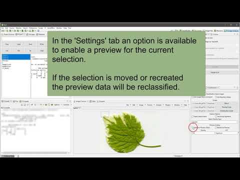
In addition the data transfer type to R can be selected (whereat most filters require a double transfer - this action will set the transfer type of images, too). It is also possible to open the default hidden feature stack which will be transfered to R (option 'Open Feature Stack') and transfer signatures according to the group membership of the ROI (option 'Use Group Signature').
If the 'Selection Preview (Train)' option is enabled a classification overlay will be generated on top of the source image with size and location of the selection. A retraining of the dataset for the preview can be enabled if the 'Retrain for Preview' option is selected. The ROI overlay will be updated dynamically if you change or move the ROI selection. Please disable the preview option (a ROI listener) or close the GUI if you recompile the plugin! The preferred LUT and opacity can be selected, too.
The enabled option "Show in ImageJ" transfers the data back to ImageJ and can be disabled if the classification result should be stored with the R scripts.
With the option "Apply ImageJ Macro" the classified image can be post-processed with an ImageJ macro, e.g., to extract and measure particles or identify image objects.

Until now Multichannel images (e.g. RGB) and Grayscale images or stacks (8-bit, 16-bit, 32-bit) can be classified. It is also possible to import images with an ImageJ macro (e.g. Landsat 8 images, see ImageJ macro example!).
For convenience images and stored ROI Manager files can be dropped on the ImageJ-Canvas view to open them. In addition a saved R workspace file can be opened, too, by dropping it on the main toolbar of Bio7. Finally a stored GUI configuration file can be opened by dropping it directly on the classification GUI.
You can download, change and customize the source with GIT.
To compile the plugin open the 'Main.java' class and compile it dynamically (use the 'Compile Java' action in the Bio7 main toolbar). The dependent classes will be compiled, too.
The 'ModelGui' SWT graphical view interface can be modified or extended with the Eclipse WindowBuilder plugin (SWT) if installed in Bio7. The Main.java class can be extended with further filters or default features.
The default R scripts and the ImageJ import macro can be changed with the R and ImageJ macro Bio7 editors.
If I want to transfer a huge image to R the following warning message about buffer size occurs: "WARNING: discarding buffer because too big awaiting.."
Solution: Increase the size of the input buffer in the Rserve preferences. Open the Rserve preferences Preferences->Preferences Bio7->Preferences R. In the Field "Rserve startup arguments" copy the following startup argument:
maxinbuf="4194304"
The max. packet size from the client to Rserve is set to 4GB in this example (maxinbuf argument in kb). Use the example size only if necessary and if you have the memory available!
The Java runtime is able to optimize memory on demand and return occupied memory to the OS. After the transfer to R the image data on the Java side in the classification process (open and transfer to R) by default is closed. If the memory settings of Java in Bio7 (see Bio7.ini file) are adjusted accordingly most of the memory can be returned to the OS and thus to R and the memory intensive classification process.
For an increased Java heap space open the Bio7.ini file in the install directory of Bio7. In the file you can change the default memory settings e.g. the initial heap size -Xms and the maximum heap space -Xmx.
For an increased Java heap space open the Bio7 package (context menu if you click on the icon) then go to Contents->MacOS and open the Bio7.ini file with a texteditor. In the file you can change the default memory settings e.g. the initial heap size -Xms and the maximum heap space -Xmx.
Example:
For instance to be able to return back much memory after image transfer use a low -Xms setting (e.g.: -Xms1024m). The maximum size for the Java Runtime (-Xmx) depends on the image size and could be adjusted depending on the available RAM (using for instance the half of the available RAM) of the OS.
In the Settings tab the datatype from Java to R can be adjusted for a less memory consumption if possible (whereat most filters require a double transfer - transfer and classification - options are: double, integer, raw).
Using the Bio-Formats library with the ImageJ macro (enable the option 'Use ImageJ Macro at Import' in the 'Settings' tab) it is possible to crop huge images to parts before the R classification process starts. The library has to be installed first as an ImageJ plugin. Bio-Formats GUI import commands can be recorded with the ImageJ macro recorder for use in the available project macro for, e.g., a specific import. If the library is used the loaded image is opened by default (can't be avoided in a macro - simply close the image after display).
The plugin uses no external Java libraries (besides ImageJ and Bio7). The filters formerly used from BoofCV and the Catalano-Framework (Gabor, Sobel gradient, Laplacian) and the texture measures are implemented in the package '_util'.
Note: the Gabor filter returns the float filter response (Catalano: a response scaled to 8-bit) - models trained with Gabor layers should be trained again.